Build Intuition About Rend-seq
Rend-seq is a form of RNA sequencing developed in the Li Lab which resolves the 3′ and 5′ ends of mRNAs with single nucleotide resolution, while simultaneouly delivering quantitative estimates of expression levels across a gene body.
This degree of resolution cannot be achieved with traditional RNA sequencing, and once you achieve it -you can interegate the context of transcription initiation, termination and RNA processing. In addition you can identify/quantify different transcription isoforms.
Rend-seq aquires its end-enriched profile by sparse fragmentation of RNA samples, followed by a size selection. The size selection ensures that we only sequence partial length transcripts. All the original 5′ and 3′ ends exist in the fragments, however the only way internal 3′ and 5′ ends will be represented is if they were randomly fragmented there, which only occurs with probability proportional to the fragmentation probability p.
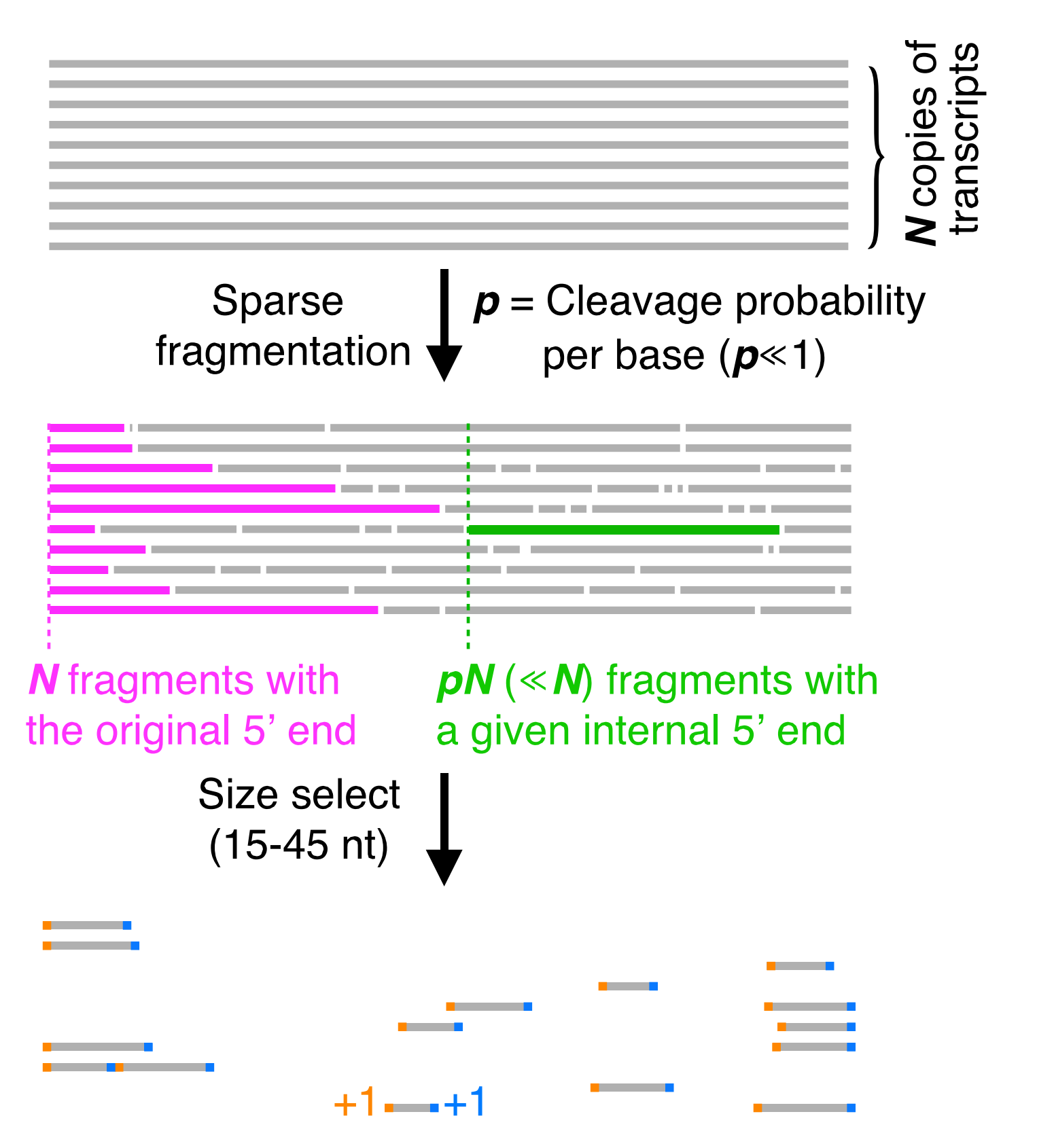
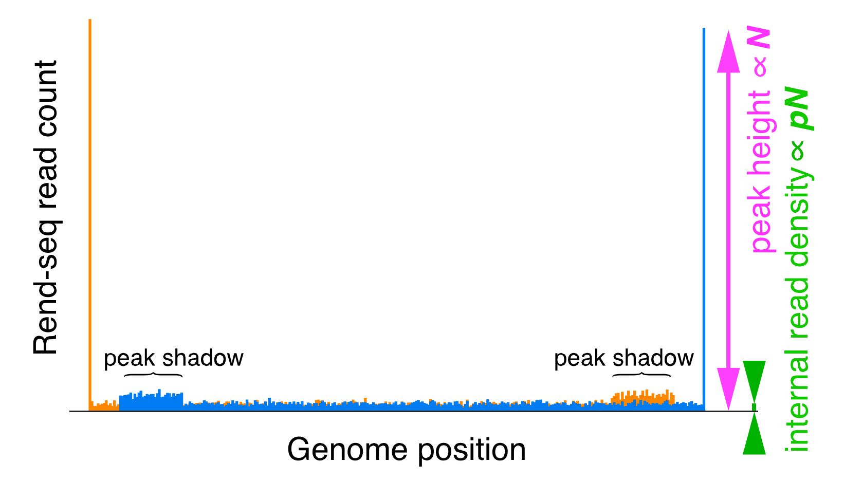
All fragments of the appropriate length are then sequenced, and their 3′ and 5′ ends are added as counts to the position they map to. The resulting data looks like 2 large 3′ and 5′ peaks, with lower internal 3′ and 5′ read density. Both peaks have a "shadow" that appears at a distance upstream/downstream that is determined by the size selection window used.
All images in this section adapted from the 2018 Cell Paper by Lalanne et al.
Illustrated Step-by-Step Rend-seq Guide
This guide is intended to help the scientist follow the Rend-seq pipeline at a molecular level. Steps are represented as diagrams of what is happening to biomolecules at each step. It was written by Jenny Cascino.
0. Start with an input of 5-20ug RNA. In this protocol we assume that the RNA has been DNase treated.
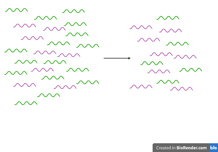
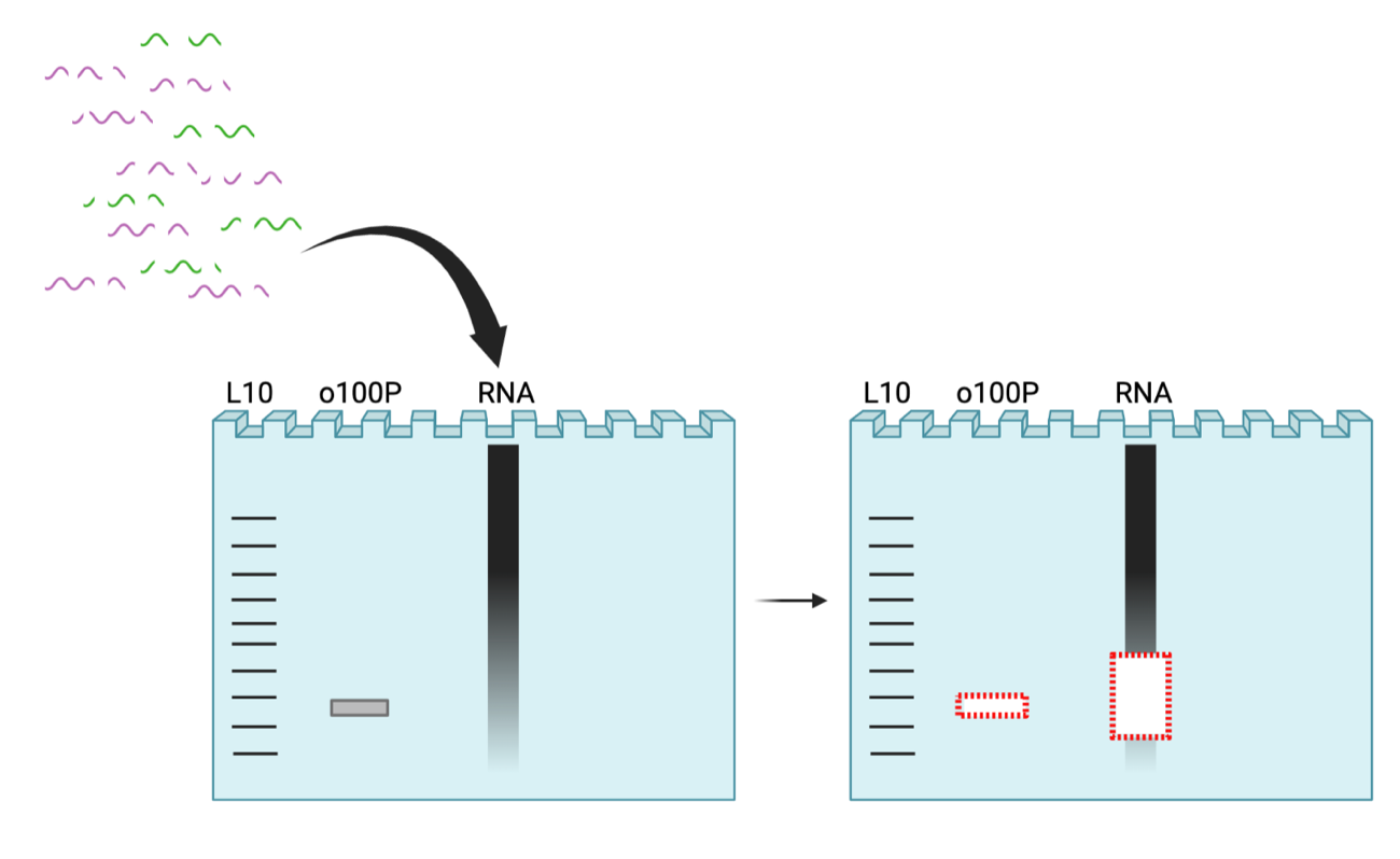
1. rRNA removal using MICROBExpress kit: green = rRNA; pink = other RNAs (tRNA, mRNA, ncRNA)
*Note: depiction is somewhat misleading. rRNA is the predominant RNA species in extraction mix, and removal merely depletes rRNA abundance. Still remains predominant RNA species after depletion.
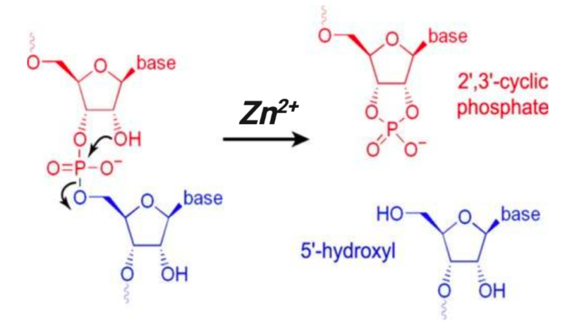
2. RNA fragmentation: 25s at 95ºC in zinc-based buffer.
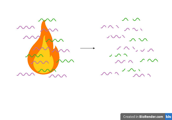
*Note: Zinc-mediated RNA cleavage has no sequence or structure specificity but is based on the attack of the 2’ hydroxyl group of ribose that leaves a 5’ hydroxyl and a 2’,3’ cyclic phosphate ester, the hydrolysis of which ultimately results in a mix of 2’ or 3’ phosphate ends. Zinc, a divalent metal cation, catalyzes the cyclization reaction that happens through a nucleophilic attack by the neighboring 2’OH (presumably by serving as an electron sink i.e. through interactions with the phosphate group that render it more electrophilic and subject to a nucleophilic attack by 2’OH that is normally not possible when the phosphate group is fully negatively charged). This is a transesterification reaction. Source for diagram and reaction chemistry.
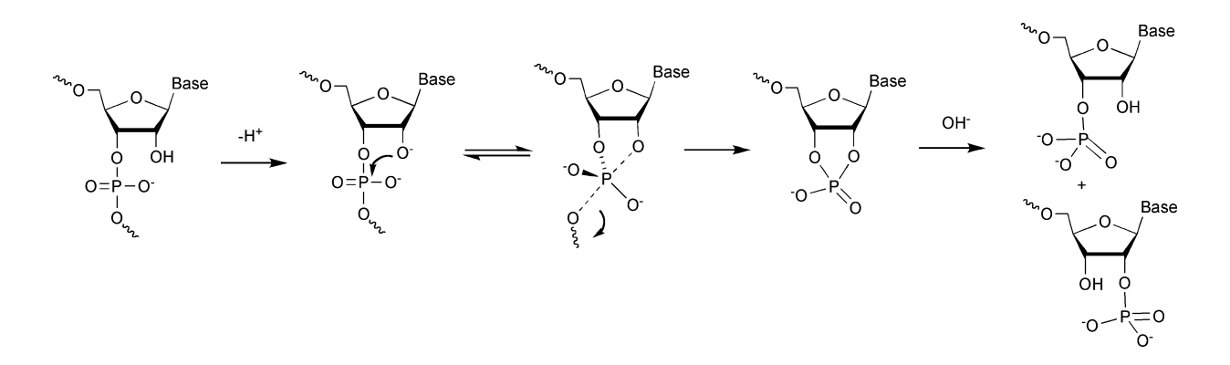
Another useful depiction:
3. Size Selection 1: Small fragments (15-45nt), 15% TBE Urea PAGE gel. Gel extract.
*Note: o199-P (28nt) serves as a positive control + size standard for next steps
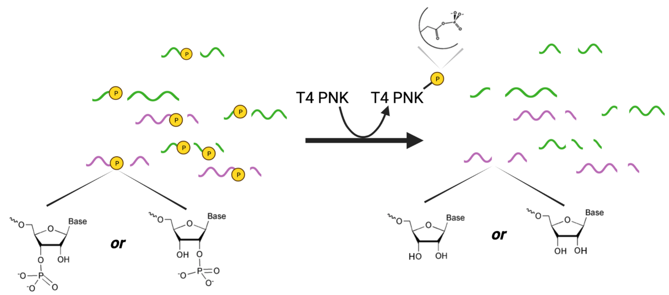
4. Dephosphorylation: Enzyme used: T4 polynucleotide kinase (T4 PNK)
Activities of T4 PNK (Source):
- 5′ phosphorylation of DNA/RNA for subsequent ligation
- End labeling DNA or RNA for probes and DNA sequencing
- Removal of 3′ phosphoryl groups “3’ end healing of RNA by T4 PNK”
- Polynucleotide Kinase also catalyzes the removal of 3´-phosphoryl groups from 3´-phosphoryl polynucleotides, deoxynucleoside 3´-monophosphates and deoxynucleoside 3´-diphosphates.
- It also may be used to dephosphorylate the 3′-ends of RNA in the absence of ATP
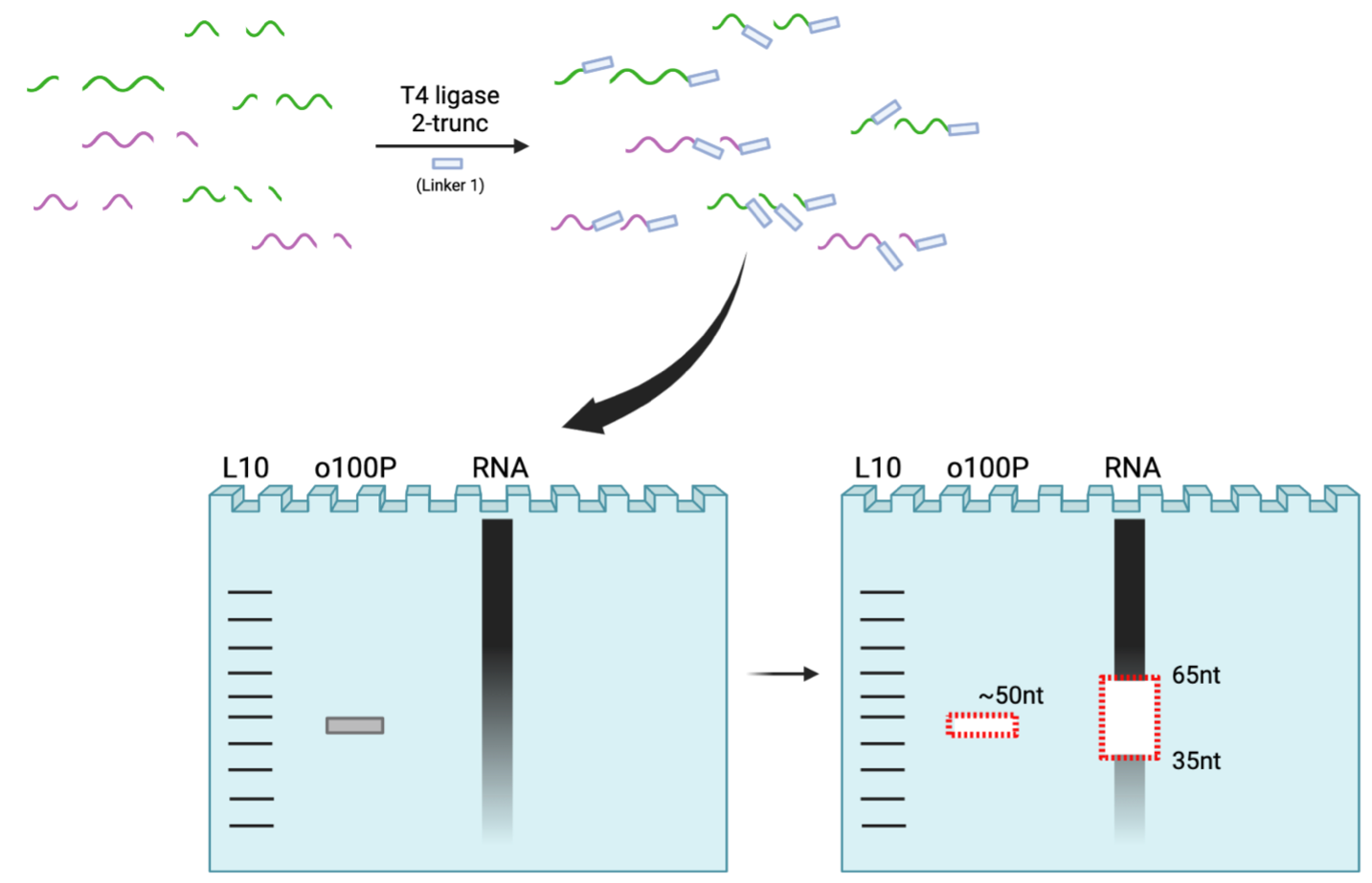
5. Ligation and size selection: 3’ end ligation of Linker 1 (19nt). 15-45nt RNA fragments + ~20nt linker size select 35-65nt
*Note: only get 3’ end ligation b/c 3’ end of Linker 1 is dideoxyC, a chain terminating nt (does not support ligation to 5’ end of RNAs)
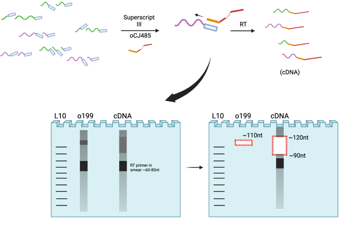
6. Reverse Transcription and Size Selection
*Note: Avoid RT primer when cutting lower bound
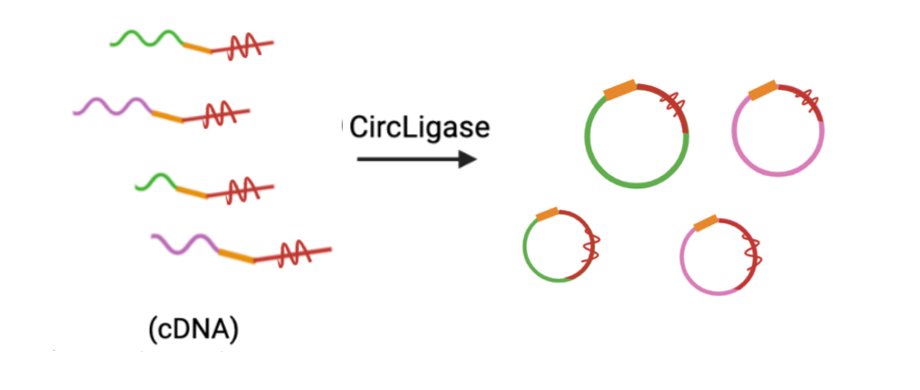
7. Circularization: circularize cDNA library to prepare for PCR-based amplification
8. PCR
Note: squiggly red line represents iSp18 linker. Indexing primer cannot extend past linker, leading to linear product that gets amplified by o231 over multiple PCR cycles.
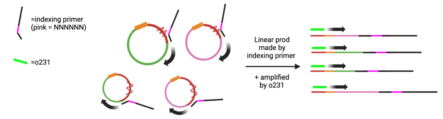
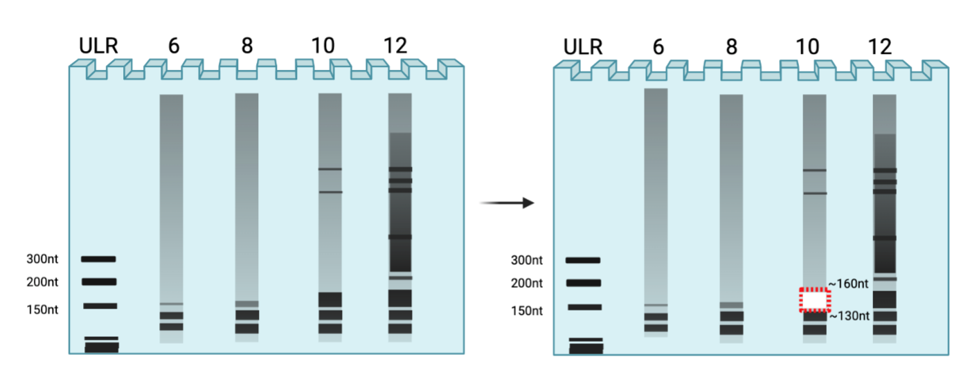
*Note: Run multiple PCRs at varying cycles usually in intervals of two: 6, 8, 10, 12 cycles. If you run multiple rounds of the last steps (i.e. ligation or RT), you may get familiar with how much input requires how many cycles and can adapt accordingly. Excise ~130-160 (3rd band, near 150nt on ultralow range ladder). You want to excise bands for cycles that yield thick band in desired range while minimizing other products.
How to analyze Rend-seq data:
Rendseq data contains a lot of information in it:
- Single nucleotide identification of the transcription start site (TSS).
- Indications of how a transcript is terminated.
- Quantitative measurements of a given transcripts abundance.
- Identificaiton of different transcript isoforms and their relative abundances.
Here we will talk about several approaches that we use to facilitate automated identification of relevant features (peaks, ramps).
We also encourage you to check out our python package rendseqwhich contains all the analysis tools discussed below to help you achieve your Rendseq analysis goals!
Peaks
First lets examine how we can call peaks.
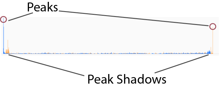
Peaks are characterized by a 1-3 nucleotide window where the read count rises sharply. There is an accopanying ~30 nt window of reads upstream or downstream (depending on strand orientation and whether one is looking at 3′ or 5′ peaks) of increased averge read height for reads of the other end type. This area is known as the peak shadow and is a result of how the sequencing protocol works (see the "Build Intuition" section for more info!). Here is a fairly straightforward example of how both peaks and peak shadows look in the wild:
Below are some details on different peak calling strategies we have implemented in our rendseqpackage.
Peak Calling with Thresholds
As the above example might suggest - peaks can often be pretty easy to spot by eye alone! One way to take advantage of the (usually clear) height differences between peak and noise floor is to set a threshold, and call everything that lies above that threshold a peak!
Because the different transcripts range several orders of magnitude in abundace one can′t simply set a read threshold and use that for calling peaks!
Instead we first transform our raw data with a modified sliding local z-score normalization, and then use our threshold to call peaks on the transformed data.
Here is how to access the z-score based thresholding peak calling functionality built into our rendseq package:
from rendseq.file_funcs import open_wig
from rendseq.zscores import z_scores
from rendseq.make_peaks import thresh_peaks

example_wig = ′some_file.wig′
reads, chrom = open_wig(example_wig)
z_score_transformed_data = z_scores(reads)
thresh_peaks_found = thresh_peaks(z_score_transformed_data)
Peak Calling with Hidden Markov Models
While the above method - ie setting a threshold on z-score transformed data - works well for many use cases, we recognize that certain assumptions in the model may not work for all data sets.
To build a more generalizable analysis tool, we have built a tool to fit your Rendseq reads using Hidden Markov Models (HMMs).
This design choice allows you to incorporate complicated distribution functions that define your peak and noise/internal distributions.
Given your distribution and transition functions, the model will return the most likely sequence of "peak" or "not peak".
Here is an example of how to do this using our rendseq package:
from rendseq.file_funcs import open_wig
from rendseq.zscores import z_scores
from rendseq.make_peaks import hmm_peaks

example_wig = ′./Example_Data/example_wig_Jean_5f_subset.wig′
reads, chrom = open_wig(example_wig)
z_score_transformed_data = z_scores(reads)
hmm_peaks_found = hmm_peaks(z_score_transformed_data)
You see that in this example we first z score transform the data, then fit the HMM using the transformed reads.
Rend-seq publications
- Evolutionary convergence of pathway-specific enzyme expression stoichiometry. Lalanne JB, Taggart JC, Guo MS, Herzel L, Schieler A, Li GW. Cell 2018.
- Functionally uncoupled transcription-translation in Bacillus subtilis.Johnson GE†, Lalanne JB†, Peters ML, Li G-W. †equal contribution. Nature 2020.
- Ubiquitous mRNA decay fragments in E. coli redefine the functional transcriptome.Herzel L, Stanley JA, Yao CC, Li G-W.. Nucleic Acids Research 2022.
- A high-resolution view of RNA endonuclease cleavage in Bacillus subtilis.Taggart JC, Lalanne JB, Durand S, Braun F, Condon C, Li GW, biorxiv 2023.
Are We Missing Something?
Note - If you have used the Rendseq protocol (or the rendseq analysis package) in your own published work and would like to be featured here, let us know! Email our dedicated mailing list at rendseq "at" mit.edu with a link to your published work.